Creeate
Jobs
Generate
Summary
Cluster
Analysis
Correlation
Analysis
Montecarlo
Analysis
Final
Portfolio
The strategy evaluation shell is an addendum to the Zorro project. Its purpose is determining the ideal parameters and functions for a given trading strategy, generating a portfolio of asset, algo, and timeframe combinations, and predicting its live perfomance under different market situations. The Zorro evaluation shell can make the best of a strategy, especially of 'indicator soup' type strategies that combine many different indicators and analysis functions.
A robust trading strategy has to meet several criteria:
The shell evaluates parameter combinations by these criteria. The robustness under different market situations is determined through the R2 coefficient, the parameter range robustness with a WFO profile (aka Cluster Analysis), the price fluctuation robustness with oversampling. A Montecarlo analysis finds out whether the strategy is based on a real market inefficiency.
Zorro already offers functions for all these tests, but they require a large part of code in the strategy, more than for the algorithm itself. The evaluation shell skips the coding part. It can be simply attached to a strategy script. It makes all strategy variables accessible in a panel, adds optimization and money management as well as support for multiple assets and algos, runs automated analysis processes, and builds the optimal portfolio of strategy variants. It compiles unmodified under lite-C and under C++, and supports .c as well as .cpp scripts.
With almost 1500 lines, the shell is probably the largest Zorro script so far, and goes far beyond other strategy evaluation software on the market. It comes with source code, so it can be easily modified and adapted to special needs. It is restricted to personal use; any commercial use or redistribution, also partially, requires explicit permission by oP group Germany. Since it creates a panel and a menu, it needs a Zorro S license to run. Theoretically you could remove the panel and menu functions and use the shell with the free Zorro version. This is allowed by the license, but would require clumsy workarounds, like calling functions by script and manually editing CSV files.
Developing a successful strategy is a many-step process, described in the Black Book and briefly in an article series on Financial Hacker. The evaluation shell cannot replace research and model selection. But it takes over when a first, raw version of the strategy is ready. At that stage you're usually experimenting with different functions for market detection and generating trading signals. It is difficult to find out which indicator or filter works best, since they are usually interdependent. Market detector A may work best with asset B and lowpass filter C on time frame D, but this may be the other way around with asset E. It is very time consuming to try out all combinations.
The evaluation shell solves that task with a semi-automated process.
|
Creeate Jobs |
|
Generate Summary |
Cluster Analysis |
Correlation Analysis |
Montecarlo Analysis |
Final Portfolio |
The first step is saving several sets of different parameter settings, named jobs. Any job is a variant of the strategy that you want to test and possibly include in the final portfolio. You can have parameters that select betwen different market detection algorithms, and others that select between different lowpass filters. The parameters are edited in the variables panel, then saved with a mouse click as a job. Since a job is just a CSV file with parameter values and ranges, you can also edit or create them directly with a spreadsheet program or a text editor.
The next step is an automated process that runs through all jobs, trains and tests any of them with any asset, algo, and timeframe used by the strategy, and stores their results in a summary. The summary is a CSV list of all jobs with their main performance metrics. It is sorted by performance, so the best performing jobs are at the top. So you can see at a glance which parameter combinations work with which assets and time frames, and which are not worth to examine further. You can repeat this step with different global settings, such as bar period or optimization method, and generate multiple summaries in this way.
The next step in the process is cluster analysis. Every profitable job in a selected summary is automacially optimized multiple times with different WFO settings. These settings are taken from - you guessed it - a separate CSV file that may contain a regular WFO matrix, a list of irregular cycles/datasplit combinations, or both. For reducing the process time, only jobs with rising equity curves - determined by a sufficient R2 coefficent - get a cluster analysis. You can also further exclude jobs by removing or outcommenting them in the summary.
After this process, you likely ended up with a couple survivors in the top of the summary. The surviving jobs have all a positive return, a steady rising equity curve, shallow drawdowns, and robust parameter ranges since they passed the cluster analysis. You can now create a set of algos from the top of the summary with a mouse click, and train them for optimal performance.
However, some of these algos might not be suited for the final portfolio. The purpose of a job portfolio is diversification, but this would not work when jobs are strongly correlated and have their drawdowns all at the same time. You want a balanced portfolio with uncorrelated algorithms. For this, run an algo comparison. It will display a chart with the equity curves from any algo. Check the curves and throw out variants with bad drawdowns, with high volatility, or with too-similar curves. After removing or out-commenting them from the summary, create an algo set again for the final balanced portfolio.
You're not finished yet. Any selection
process generates selection bias. Your perfect portfolio is
picked from a multitude of job variants, and will likely
produce a great backtest. But will it perform equally well in live trading? To
find out, run a Montecarlo
analysis. This is the most important test of
all, since it can determine whether your strategy exploits a real market inefficiency
or is just a product of selection bias. If
the Montecarlo analysis fails with the final portfolio, it will likely also fail
with any other parameter combination, so you need to run it only at the
end. If
your system passes Montecarlo with a p-value below 5%, you can be relatively
confident that the system will return good and steady profit in live trading.
Otherwise, back to the drawing board.
This manual is split in two parts. The following sections deal with the
user interface of the shell. For a quick usage example, scroll down to the
end. Attaching the shell to an existing strategy is
described in the tutorial.
When you start a strategy with attached shell, the [Result] button will change to [Start], a new menu will be available under [Action], and a panel with the current parameter and variables of the strategy will pop up:
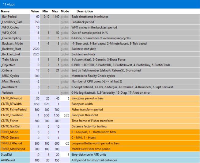
The panel and menu are the reason why a Zorro S license is required, since panel functions are not supported by the free version. The variables in the panel are divided in three sections.The general system settings, common for all strategies, are in the grey area. The strategy variables specific to a certain algorithm are in the area with red or yellow colors, where any algorithm has its individual color. The strategy variables common to all algorithms are in the blue area.
Every variable is represented by a row in the panel. The first field is thje variable name. The Fixed field can be active (x) or disabled (o). It can be switched between the states with a mouse click. If a variable value is fixed, it overrides the value from a saved job or from optimization. By default, the system variables are fixed, the strategy specific variables are not.
The Value, Min, and Max fields contain the default value and range (if any) of the variable. You can edit any field and change its value. Edited values in the panel are remembered at the next start. Changes are indicated with a white background. Exceeding the valid range is allowed, but indicated with a red background.
The Step field is for variables that can be optimized. A negative step width establishes a percent increase, as recommended with large optimization ranges. If the step width is set to 0, the variable is not optimized, and gets its default value instead..
The system settings in the grey area are mostly self explaining:
| _Bar_Period | The basic bar period from which the time frames are derived. Must be unchanged for all jobs of a session. |
| _Lookback_Bars | The lookback period in bar units. |
| _WFO_Cycles | Number of WFO cycles in the backtest, including the last cycle for live trading. Rule of thumb: Use 1-2 cycles per backtest year. |
| _WFO_OOS | Out-of-Sample period for WFO, in percent. |
| _Oversampling | Number of oversampling cycles with differently sampled price curves in the backtest. Must be unchanged for all jobs of a session. |
| _Backtest_Mode | -1 for a 'naive' backtest with no trading costs, 0 for the script default, 1 for a realistic bar based backtest, 2 for a minute based backtest, 3 for a backtest with tick-based history. Must be the same for all jobs of a session. Historical data in the required resolution must be available. |
| _Backtest_Start | Start year or date of the backtest. Use at least 5, better 10 years for the test period. Must be the same for all jobs of a session. |
| _Backtest_End | End year or date of the backtest. Must be the same for all jobs of a session. |
| _Train_Mode | 0 Script default, 1 Ascent (fastest), 2 Genetic, 3 Brute Force (see TrainMode). Results of genetic optimization can differ on any training due to random mutations. |
| _Objective | Training objective, aka 'fitness function'. 0 PRR (default), 1 R2*PRR, 2 Profit/DD, 3 Profit/Investment, 4 Profit/day, 5 Profit/trade. For the metrics, see performance. |
| _Criteria | The field number by which the summary is sorted and the profiles are generated. 0 no sorting, 7 Net Profit, 13 Win rate, 14 Objective, 15 Profit factor, 16 Profit per trade, 17 Annual return (default), 18 CAGR, 19 Calmar ratio, 20 Sharpe, 21 R2 coefficient. See performance for details about the metrics. |
| _MRC_Cycles | Number of cycles for the Montecarlo 'Reality Check' analysis (default 200). Results differ from run to run due to randomizing the price curve, therefore more cycles produce more precise results. |
| _Max_Threads | Number of CPU cores to use for WFO (0 = single core), or number not to use when negative (f.i. -2 = all cores but 2). Must be unchanged for all jobs of a session. Using multiple cores is recommended for faster training. |
| _Investment | Method for calculating the trade size after algos have been created. 0 Script default, 1 Lots slider, 2 Margin slider, 3 Margin * OptimalF, 4 Percent of account balance, 5 Percent * square root reinvestment. At 3 or above, OptimalF factors are generated and affect the margin. 4 and above reinvest profits and should only be used in the last stages of development. |
| _Phantom | Activate equity curve trading by setting the time period between 10..50. A falling equity curve is detected and trading is suspended until the market turns profitable again. |
| _Verbose | Set to 0 for no logs and reports, 1..3 for more verbose logs, 17 for halting on any error. The more verbose, the slower the test. Critical error messages are collected in Log\Errors.txt. Performance summary reports are always generated, regardless of this setting. |
After starting the script in [Train] mode, a click on [Action] opens a dropdown menu, like this:
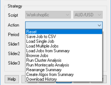
| Reset | Reset all variables to their defaults, and remove all loaded jobs and algos. |
| Save Job to CSV | Save the current panel state with all variables to a job file in CSV format, in a folder of your choice (Job by default). If the system has no own algos, the job file name will be later used for the algo names, so don't use a complex or long name. |
| Load Job to Panel | Load a set of variables from a job file to the panel. A click on [Start] will train the job and store its result in the Summary. Any trained job will also store its 'papertrail' of charts, logs, and reports in a subfolder named after the job. |
| Load Job with Variants | Generate jobs from a single job file with all asset, algo, and timeframe variants. A click on [Start] will train all job variants and store their results in the Summary and in their 'papertrail' folders. |
| Load Jobs from Folder | Select a folder by clicking on a job file inside. All jobs in that folder are loaded, together with all their asset, algo, and timeframe variants. A click on [Start] will train all jobs and store their results in the Summary and in their 'papertrail' folders. |
| Add Jobs from Folder | Select a Summary generated by previous training. All jobs in the same folder that are not already listed in the summary are loaded. A click on [Start] will train the jobs and add their results to the Summary and their 'papertrail' folders. |
| Load Best from Summary | Select a Summary generated by previous training. All jobs listed in that summary with a sufficient number of trades, profit factor, and R2 coefficient are loaded. The thresholds are defined in eval.c. Jobs can be excluded by adding a '#' hash in front of the name. |
| Load Marked from Summary | As above, but load all jobs marked with a '*' asterisk in front of the name in the summary. |
| Copy Jobs to Folder | Select a non-empty folder by clicking on a file inside. All currently loaded jobs are copied into that folder. |
| Run Cluster Analysis | Run a WFO cluster analysis for all loaded jobs, with WFO offsets and OOS periods defined in a CSV file. Several files with various combinations of offsets and periods are included. For any WFO cycles / OOS period combination, the resulting performance metrics are stored in a Cluster summary. For files containing a regular NxM cluster matrix, the returns are displayed in a heatmap, otherwise in a WFO profile. |
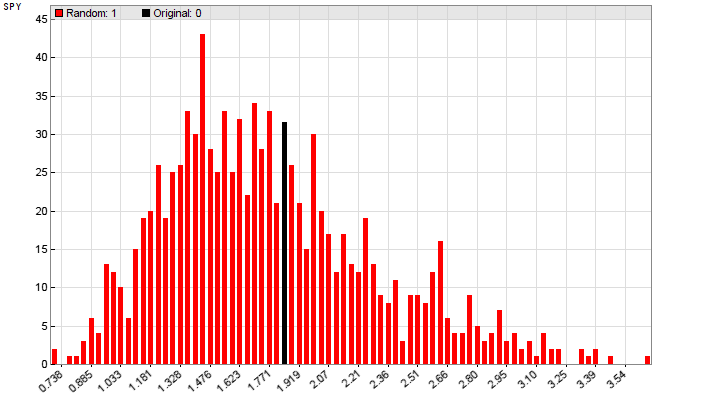
| Run Montecarlo Analysis | Run a Montecarlo 'Reality Check' with the current parameters and shuffled price curves. A reality check can tell whether the WFO performance was just luck, or was caused by a real market inefficiency. The resulting performance metrics are stored in a MRC summary, and the results are displayed in a histogram together with the original result with unmodified price curve. Depending on the resulting p-value, the backtest performance is qualified as significant, possibly significant, or insignificant. |
| Rearrange Summary | Re-sort the entries in the summary if _Criteria was changed, or if new jobs were manually added to the summary. |
| Create Algos from Best | Select a summary generated by training jobs. All jobs from that summary with a CA result > 60% are selected for the final portfolio. Their variables, assets, algos, and time frames are stored in Data\*_algo.bin, a backup is stored in *_algo.bak. This file is automatically loaded at start, so that training, testing, and trading will now use the algo porfolio. To remove the algos, use Reset. |
| Create Algos from Marked | As above, but select all jobs marked with a '*' asterisk in front of the name in the summary. |
| Run Algo Comparison | Generate a chart with the equity curves from any algo of the portfolio. If you don't like an equity curve, remove the job by outcommenting it with a '#' in the summary, then create the algos again. |
| Download History | Open the Zorro Download Page for getting historical data. |
When no job was loaded, clicking on [Start] will just start a test or training run with the current variable settings in the panel. After a successful backtest, the performance report will open in the editor, and the chart viewer will display the price curve, the trades, and the equity curve. Train mode will always use walk forward optimization, even when none is defined in the script. Test mode will only run a backtest; so the strategy should have been trained before. After changing any variable, train again. If a variable range was exceeded or historical data was missing for the selected backtest period, you'll get an error message. Training errors will store the error message in Log\Errors.txt and abort.
When one or more jobs are loaded, a click on [Start] will train and test all of them in all their asset, algo, and timeframe variants. Their logs, performance reports, and charts will be stored in a subfolders named after the job. In this way training and testing jobs leaves a 'perpertrail' that allows evaluating individual results. Instead of the performace report, a summary report will open in the editor.
The summary report appears when multiple jobs are trained or tested. Any job in any asset, algo, and timeframe variant generates a record in the summary. The summary is sorted, with the best jobs, selected by the _Criteria variable, at the top. It is stored in CSV format, so it can be further evaluated in a spreadsheet program.
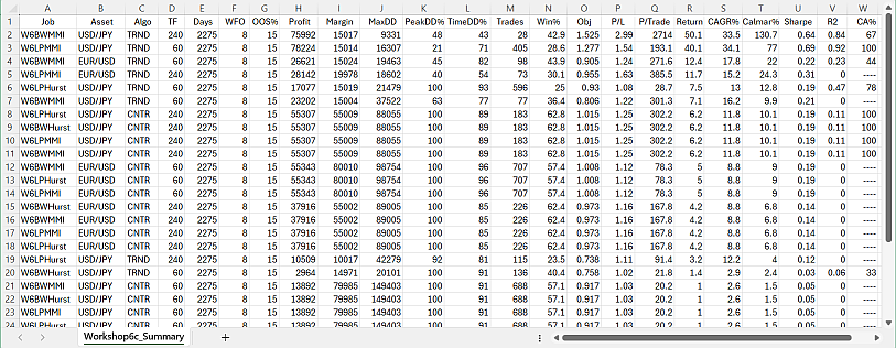
The fields:
| Job | Job name |
| Asset | Asset used by the job. |
| Algo | Algo used by the job (if any). |
| TimeFrame | Time frame of the job, in minutes. |
| Days | Total days of the backtest, not counting lookback and training. |
| WFO | Number of WFO Cycles |
| OOS% | Out-of-sample period in percent |
| Profit | Sum of wins minus sum of losses minus trading and margin cost. |
| Margin | Amount required for covering the maximum open margin |
| MaxDD | Maximum equity drawdown from a preceding balance peak |
| PeakDD% | Max equity drawdown in percent ot the preceding peak |
| TimeDD% | Time spent in drawdown in percent of backtest time |
| Trades | Number of trades |
| Win% | Percent of won trades. |
| Obj | Backtest return of the objective function. |
| P/L | Profit factor, the sum of wins divided by sum of losses |
| P/Trade | Average profit per trade |
| Annual% | Annual net profit in percent of max margin + max drawdown. |
| CAGR% | Annual growth of the investment in percent. |
| Calmar | CAGR divided by max drawdown in percent. |
| Sharpe | Annualized mean return divided by standard deviation |
| R2 | Equity curve straightness, 1 = perfect |
| CA% | Percentage of runs that passed the cluster analysis. |
The meaning of most performance metrics can be read up under performance report, but the metrics in the summary are unadjusted. This means that drawdown, annual return, and Calmar ratio depend not only on performance, but also on the length of the backtest period.
The test results for any job are automatically stored in subfolders of the selected job folder. The subfolders are named after the job, its asset, its algo, and its timeframe. In this way any job leaves a 'papertrail' of of text, CSV, image, and html files from its training and test runs. All reports can be opened with a plain text editor such as the included Notepad++. The .csv files can also be opened with Excel, and the chart images with an image viewer like the included ZView.
Aside from the summary and the CA or MA charts, the following reports are produced when jobs are processed (for details see exported files):
*.txt - the last performance report.
*history.csv
- the performance history of the job. Any test or training run adds a line to
the history.
*.png - the chart with
the equity curve, trades, and indicators.
*.htm - a page with parameter charts that
visually display the effect of parameters on the performance.
*.log - the
event log of the backtest.
*train.log
- the training log with the objective results for all
tested parameter combinations.
*pnl.csv -
the equity curve of the backtest, for further evaluation.
*trd.csv
- the trade list of the backtest, for further evaluation.
*par.csv
- the results of genetic or brute force training runs, for further evaluation.
Log\Errors.txt - the last
errors encountered (if any) while training or testing.
Cluster analysis (CA) can be performed either with the current settings and algos, or with a selected job and its variants, or with promising jobs loaded from the summary. In the latter cases its results are stored in the CA% field of the summary report. For reducing process time, only jobs with profit factor and R2 value above predefined limits (1.25 and 0.25) will be loaded from the summary. And only jobs with more than 75% positive CA runs will be taken over to the next step, the algorithm selection.
Dependent on the selected cluster template, Cluster analysis will generate either a WFO profile or a heatmap: The cluster template is a CSV file with an arbitrary number of WFO cycle / OOS period combinations, like this:
WFO,OOS%
-4, 25
-3, 22
-2, 20
-1, 18
0, 15
1, 12
2, 9
3, 7
4, 5
The first column are offsets to the value of the _WFO_Cycles variable, the second column are the OOS periods in percent. Any offset/period combination generates a performance values that is determined by _Criteria and displayed in a profile diagram, which pops up in the chart viewer:

WFO profile,
from a non-matrix cluster analysis. Y axis: _Criteria, X axis:
line number in the template.
Usually, the cluster template will be a regular matrix, like this (for a 5x5 matrix):
WFO,OOS%
-2, 5
-2, 10
-2, 15
-2, 20
-2, 25
-1, 5
-1, 10
-1, 15
-1, 20
-1, 25
0, 5
0, 10
0, 15
0, 20
0, 25
1, 5
1, 10
1, 15
1, 20
1, 25
2, 5
2, 10
2, 15
2, 20
2, 25
This will produce a heatmap as below. The X axis is the number of WFO cycles, the Y axis is the OOS period in percent. The numbers in the fields are the resulting strategy performance by _Criteria.
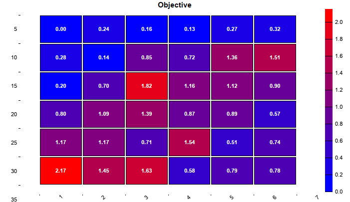
WFO heatmap, from cluster analysis with a regular matrix
The color of the fields represents the performance. You want as much red
fields in the heatmap as possible. The example above, with the Pessimistic Return Ratio (PRR) as metric, has only 13 red fields out of 25. This job would not pass the
75% CA threshold.
The goal of evaluation is creating a balanced portfolio from optimal components. Create Algos from Best will generate a portfolio from the best job variants with at least 60% CA and 1.25 profit factor, and store it in "*_algo.bin" in the Data folder. This portfolio is then loaded at start, and further test or training operations are applied to the whole portfolio unless it is reset or something else is selected. The algo/asset/timeframe components are listed at start, like this:
Algo TRND_2 (EUR/USD, 60M)
Algo TRND_5 (USD/JPY, 60M)
Algo CNTR_7 (USD/JPY, 240M)
Algo CNTR_8 (EUR/USD, 240M)
Algo CNTR_9 (USD/JPY, 240M)
Algo CNTR_10 (USD/JPY, 240M)
The numbers refer to the records in the summary.
After creating and training a portfolio of algos, run an algo comparison in [Test] mode. It produces a chart like this:

You can now identify equity curves that you don't like - there are several in the above example chart - and remove them from the summary, or outcomment them. The numbers in the algo names are the line number in the summary.
Montecarlo Analysis, aka 'Reality Check', is normally only applied to the final strategy after algos have been generated. It produces a histogram of results from randomized price curves (red) and from the original price curve (black). This one below (from the 'placebo system' in the Financial Hacker article) indicates that you better don't trade that system live, even though it produced a great walk-forward analyis.
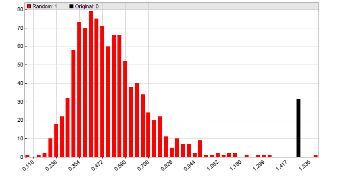
Another Montecarlo histogram from a real stragegy that generated less walk-forward performance than the 'placebo system', but a lot more performance in live trading since it exploits a real market inefficiency:
More about cluster analysis and Montecarlo analysis can be found on
financial-hacker.com/why-90-of-backtests-fail. Make sure to train the
portfolio again after the Montecarlo analysis, since the original training data
have been overwritten by the process.
Naturally, training hundreds of jobs and variants will take its time. For
highest speed, activate multiple threads, code in C++, and use the 64 bit Zorro
version.